The 2023 NFL regular season is knocking on the door, and one of the most discussed questions during the season will be which teams are actually good. With only 17 games, different schedule strengths and a lot of games decided by only one score, the win-loss record of a team — while ultimately deciding one's playoff fate — can only do so much when it comes to separating the signal from the noise.
And even beyond the luck that is inherently baked into wins and losses, the underlying points themselves can also come with a lot of variance. Especially with teams going for it more on fourth down, a few inches will more and more often be the difference between zero or seven points on the board.
The goal of this article is to develop a metric that looks at the signal of driving down the field prior to that goal-line attempt instead of focusing on the singular event of a fourth-down attempt. Concretely, we want to separate the signal from the noise in points scored and conceive a metric called noise-canceled score, which is supposed to shed a better light on how well two teams played or are playing.
Expected drive points
We want to create a metric that works on a drive basis, allowing us to compute the expected score at any time in the game. The key is to give an offense credit for how far and efficiently they moved the ball on a drive, regardless of starting field position.
Quantifying how far the ball was moved on a drive is easy at first glance, as we can just measure the yards from the starting point to the endpoint of the drive. However, this comes with two problems:
- What’s the “endpoint” of a drive? That might be trivial on a scoring drive, but definitely not for other sorts of drives. When the ball is moved from a team's own 20-yard line to their own 40 and then the offense has a two-yard run on first down, a 10-yard sack on second down and an incompletion on third down, how do we define the endpoint? Is it the own 40? Or the own 42 (after the two-yard run)? Or the own 32 (where the drive ended on third down)? We could define it to be the furthest point, but which point is further in terms of scoring points? First-and-10 at the 40 or second-and-8 at the 42?
- A similar problem arises with field goal drives. How do we define the furthest point of the drive that went deep inside the red zone but ended on a field goal after unsuccessful goal-line attempts?
- Our goal was to conceive a noise-canceled score. That is, we want point values — not yard values.
The good news is that the answer to the third point automatically answers the two former points, too.
We are going to measure the current value of a drive in terms of points by training a model that computes the likelihood of each possible drive outcome in terms of points scored (negative two points, zero points, three points or seven points) based on the situation (down, distance, field position and time left). Using this, we can assign a point value to any point of a drive, namely the points an NFL team is expected to score on that drive from that point. Here is how it looks with 10 yards to go based on down and field position.
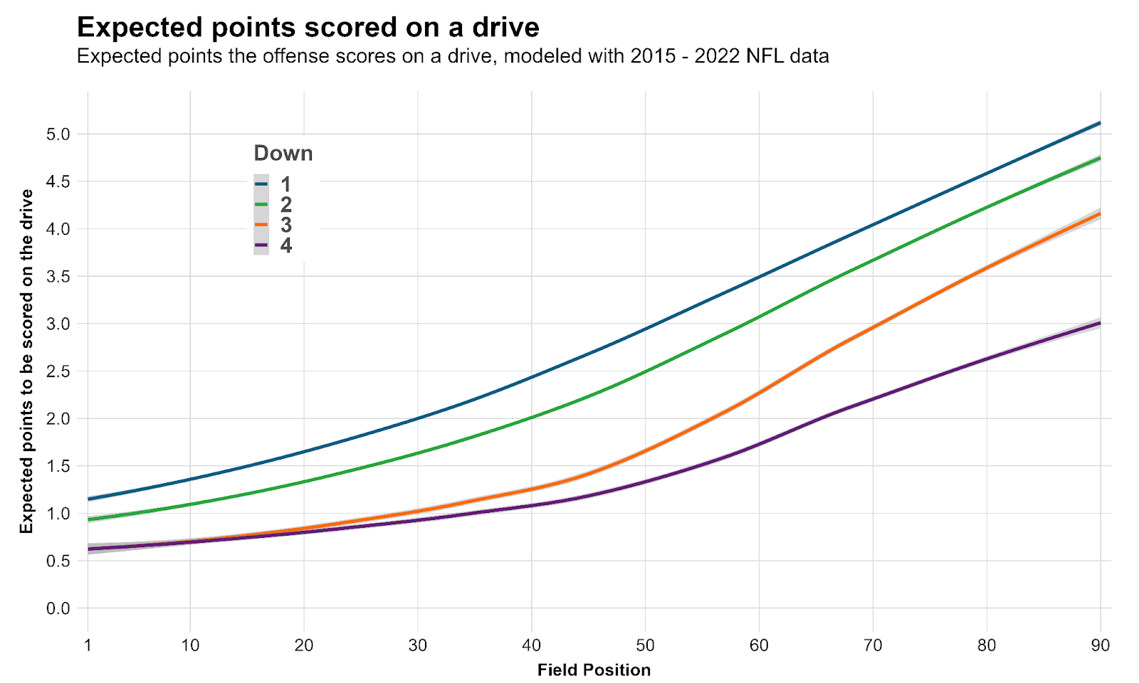
We now have a natural way to define the endpoint of a drive: It’s just the drive's highest point at any moment. This is not necessarily the last play of the drive or the furthest point in terms of field position. For example, if a team has the ball in the red zone on first down but throws an incompletion, runs for one yard on second down and then fails on third down en route to scoring a field goal on fourth down, the “endpoint” of the drive would have been reached at first down, despite the team having been closer to the end zone on third-and-9. As the graph shows, the drive would’ve been worth more than 4.5 points at this point (which is more than the field goal the team eventually scored).
To summarize, if a team starts on its own 20-yard line (1.63 expected drive points) and ends up with a first-and-10 on the opposing 10-yard line (5.03 expected drive points), the offense gets credit for the difference — 3.40 points. However, this is just the starting point of our metric. Let’s move on to the fine-tuning.
Measuring the efficiency of moving the ball
In the introduction of this article, we claimed that we would not only measure how far the ball is moved but also how efficiently the ball is moved. Obviously, an offense chaining together five conversions on first-and-10 to move the ball from their own 20 to the opposing 10-yard line is a more impressive feat than moving the ball the same 70 yards via multiple third- (or even fourth-) down conversions. In particular, the former is a more repeatable feat, whereas the latter had a lot of potential to go wrong. Since our goal is to separate the signal from the noise, we definitely want to quantify the difference between these two hypothetical drives.
The difference between those two drives is to be found in the series within the drive. A series is a series of downs, starting with first down and then potentially going to second through fourth down. Whenever a team moves the sticks, the series was successful and a new series (of downs) begins. If a series goes through first-and-10 and second-and-3 before it’s converted to a new series, that’s more impressive than a series going through first-and-10, second-and-9 and third-and-6. How do we quantify that?
A natural way to do this is by using our drive points model from above to predict the average drive points during a series of downs (until the chains are moved or the ball is punted away/turned over). For example, let us consider an offense on first down at midfield. This is worth 2.88 points.
In the first case, the offense might convert on first down. There was only one play in the series, so the points average during the series was 2.88.
In another case, the offense might also convert but go through second-and-9 and third-and-9. These plays from the opposing 49-yard line are worth 2.50 and 1.65 points, respectively. The points average during the series was 2.34.
We can call these numbers the series point value. By computing the series point value of every historic series in the NFL of the past eight years, we get the average series point value of a series that starts on first-and-10 at a given field position. We find that the number for a series starting at midfield is 2.62. In particular, the offense converting on first-and-10 was 0.26 points more efficient than average on that series, while the offense going over third-and-long was 0.28 points less efficient than average on that series.
For one drive, we can simply add up these deviations for every series and end up with a cumulative series deviation that describes whether a team moved the ball more or less efficiently than average. Note that we only consider the deviation on series that were ultimately converted, because we're not measuring whether the ball was moved (the drive endpoints already do that), but how efficiently it was moved when it was moved. In other words, it’s not inherently correlated to how far the ball was moved.
This method quantifies the efficiency of moving the ball in terms of points in a natural way. It is the perfect way for us to credit offenses for moving the ball efficiently and discredit offenses that moved the ball in a way that is more prone to failure because the drive was close to coming to a stop multiple times.
Accounting for singular events
Singular events of a drive are usually how they started or ended: Interceptions, fumbles, (missed) field goals, touchdowns and safeties. Some of these events are worth a lot of points in a football game. The average turnover is worth between four or five points, and turnovers that are returned for a lot of yards or even a score can be worth more than seven points. The swing on a field goal is obviously three points, and the value of a touchdown and safety are well known to be seven and two points, respectively.
A lot of these events are very noisy, though. It is common knowledge by now that turnovers appear much more randomly than most people believe, and the same is true for missed field goals. Even touchdowns can be noisy. A fourth down at the two-yard line is basically a 50-50 proposition, but the result swings the game by seven points.
While often noisy, these things are still meaningful. Good teams score more touchdowns in similar situations, and bad teams will throw more interceptions in similar situations. Good kickers will obviously miss field goals less often than bad kickers. Hence, we should account for them, but we should downgrade their effects.
Turnovers, missed field goals and safeties will simply add a negative value to each drive. For turnovers, we differentiate between interceptions, fumbles on carries or after receptions and sack fumbles. For interceptions, in particular, we look at the average negative expected points added value of an interception with a given pass depth in a given situation and let the penalty be some multiple of that.
We found that the following values yield the highest predictiveness:
- Interceptions: 40% of the negative value they usually have
- Fumble on a carry or reception: -1 points for the offense
- Sack fumble: -2 points for the offense
- Missed field goal: -1 point for the offense
- Safety: -1 points for the offense
An interesting result of the study is that among the two extreme choices of 1) singular events count as much as they count toward actual scoring, and 2) singular events are completely ignored, the second choice actually led to a higher predictiveness. Nevertheless, the best results are obtained by finding the best mix between both choices.
Touchdowns will be treated differently, as they will add to the endpoint of the drive. If the maximum drive points of a drive were five and a touchdown was scored, the new endpoint of the drive will be a weighted average of five and seven:
Drive endpoint value = TD_WEIGHT * 7 + (1 – TD_WEIGHT) * 5
A weight of zero would mean that we completely ignore the touchdown-scoring play. A weight of one would mean that every touchdown drive is credited with the full seven points.
We found that the highest predictive power occurs for a TD_WEIGHT of 0.9. In other words, touchdowns should definitely count for something, but the difference between scoring a touchdown or kicking a field goal at the goal line will not be four points like in the “real” scoring system. For instance, if an offense earned a first down from the 12-yard line (worth roughly five points), the drive will end with five drive points if it stalls right there and with 6.8 (weighted mean between five and seven) if they go on to score a touchdown on the very next play.
Other than for the negative singular events, it turned out that completely ignoring touchdowns and just looking at the furthest point before the touchdown would significantly decrease the predictive power of our metric. This suggests that capitalizing on good drives by scoring touchdowns is indeed a skill that any holistic offensive metric has to appreciate. However, the key of our metric is that if a team fails to score a touchdown, it still gets credit for a potentially good drive.
Bringing it all together
After our preliminary work, the final formula for the points an offense gets credit for on a drive (and the defense gets blamed for) is very easy:
Drive Value = Drive endpoints (incl. potential TD bonus) – Drive start points + 0.5 * cumulative series deviation + penalty for singular drive endings
The factor 0.5 for the cumulative series deviation was conceived by, again, looking for the highest predictive power. The fact that this number is greater than zero shows us that the efficiency when moving the ball is meaningful, but the fact that this number is smaller than one shows us that moving the ball at all is still the bread and butter of an offense.
How do we know this is a useful metric?
Our metric has descriptive usefulness. First, it correlates highly with point differential in-sample. The correlation between the score of a game and the noise-canceled score of a game is 0.88.
Furthermore, it seems to pass the eye test: The best team according to noise-canceled score differential since 2015 was the 2019 Baltimore Ravens. The best offense according to noise-canceled points scored was the 2018 Kansas City Chiefs. And the best defense was the 2019 New England Patriots.
Generally, it does a better job of differentiating offense and defense from a scoring perspective. By the nature of its computation, offenses are solely responsible for scoring noise-canceled points and defenses are solely responsible for preventing opposing noise-canceled points. For the actual score of a football game, offenses are also responsible for the opponent not scoring via avoiding turnovers and bad starting field positions for their own defenses.
Vice versa, defenses can help put up points by either doing it directly via returning turnovers or by setting up the offense with good field position. We can give some evidence by looking at in-sample correlations to offensive and defensive EPA per play over the course of a season. (The sign of the correlation coefficients in the table is chosen such that good things show in the same direction. In other words, a higher EPA per play figure on offense would correlate positively with fewer points allowed.)
| Off EPA/play | Def EPA/play allowed | |
| Points scored | 0.85 | 0.16 |
| Noise-canceled points scored | 0.92 | 0.02 |
| Points allowed | 0.23 | 0.76 |
| Noise-canceled points allowed | 0.07 | 0.87 |
The consequence is that other than actual point differential, this metric allows us to separate offense and defense. That is, if one team beats their opponents by an average of 23-20 and another team by an average of 26-23, we can conclude that the latter team is better on offense and worse on defense than the other team.
As an example, the 2018 Bears and 2017 Jaguars were among the best defenses in recent history. These teams scored 421 and 417 points respectively, which ranks 60th and 68th among all 256 teams in a season since 2015. That would suggest they fielded top-10 offenses.
However, when looking at noise-canceled points, these two teams scored only 377 and 376 points, respectively, ranking 116th and 120th. This comes closer to the truth that these were mediocre offenses carried by extraordinary defenses (they rank second and third in noise-canceled points allowed over the past eight seasons).
From a predictive standpoint, our metric is useful if it does two things:
- It is stable and predicts future team performance at least as good as the baseline metric. Since our metric is a score, the baseline metric is, of course, the “real” score — the point differential.
- The information we threw away is much less stable and much less predictive.
First of all, our noised-canceled score metric is quite stable, with the correlation between the first and the second half of the season for teams since 2015 being 0.47. This is the same number we find for the point differential itself. When testing the stability of what we threw away (i.e., the difference of point differential and noise-canceled point differential), we find a correlation of only 0.13.
We found the following out-of-sample correlation when comparing the first half and the second half of the season of each team and season since 2015.
| First half metric | Second half metric | Correlation (R-value) |
| Point differential (PD) | Point differential | 0.47 |
| Noise-canceled score (NCS) | Point differential | 0.48 |
| The difference of NCS and PD | Point differential | 0.22 |
This means that our metric predicts future team performance just as well as point differential — and maybe even better. This makes it an inherently useful metric to look at. Meanwhile, the difference between the noise-canceled score differential and the actual point differential (the information we threw away in the metric) has only very little predictive power.
Since our metric is computed on a drive basis, we can also compute it at halftime of each game. Since 2015, 1,159 NFL games were close at halftime (within one score).
In these games, the team that “led” the game at halftime by our noise-canceled score metric went on to win the game at a 1% higher rate than they were supposed to based on the halftime score and whether they got the ball to start the second half.
Which recent games were flipped?
The greatest difference between the actual score and the noise-canceled score of the past three years happened in the 2020 game between the Miami Dolphins and the Los Angeles Rams, a contest that the Dolphins won 28-17 with the help of three touchdowns on defense and special teams. The Dolphins couldn’t move the ball on offense, gaining less than three yards per play. The Rams moved the ball at an average rate, and that should’ve been enough to win the game in a low-scoring affair without the turnovers. Our noise-canceled score had this game at 18-8 for the Rams.
The greatest difference last season appeared in a game between the Chicago Bears and the Washington Commanders in Week 6. The Commanders couldn’t get much going, and the Bears nearly gained twice as many yards. By our noise-canceled score, the Bears should have won 23-13. However, an interception, a fumble and zero touchdowns on three red-zone trips had the Bears losing this game 12-7.
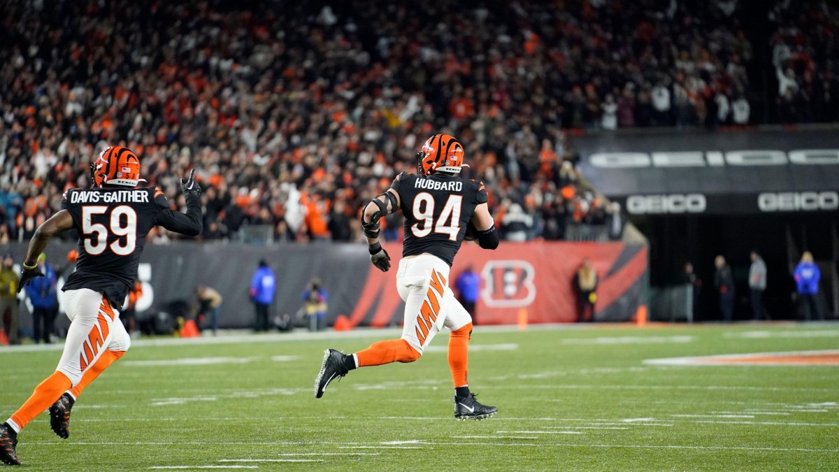
You might not have remembered the Bears-Commanders game, but most readers will still remember last season’s wild-card game between the Ravens and Bengals. When a team wins a close game after a 14-point swing — Sam Hubbard’s fumble return — it’s safe to say that the other team probably should’ve won by our noise-canceled score metric. Indeed, the metric had this game as a 24-18 win for the Ravens. Given that the game ended 24-17, the difference is almost exactly the difference between scoring a touchdown at the goal line instead of the Bengals recovering a fumble and returning it for six.
Were the Chiefs a deserved Super Bowl winner?
The short answer is yes. The long answer is that the Philadelphia Eagles would have also been a deserved Super Bowl winner, because, in fact, we have the Chiefs with 29.57 noise-canceled points and the Eagles with 29.49 noise-canceled points. In other words, the game was a tie, according to our noise-canceled score.
Looking at prior playoff games, the Chiefs beat the Bengals 23-17 and the Jaguars 29-20, according to our noise-canceled score. Both games looked closer on the scoreboard, hence one can conclude that the Chiefs were definitely well-deserved Super Bowl winners and didn’t get there through fluky games.
Conclusion
Nobody is going to file a petition to determine the winner of a game by an advanced metric. Nevertheless, we were able to create a scoring metric that has useful descriptive properties such as separating offensive prowess from defensive prowess and successfully manages to separate the signal from the noise, as our analysis of its predictiveness shows.
Our new metric helps us paint a better picture of a game and allows us to better understand how well both teams played.